
Anticlustering partitions a pool of elements into clusters (or anticlusters) with the goal of achieving high between-cluster similarity and high within-cluster heterogeneity. This is accomplished by maximizing instead of minimizing a clustering objective function, such as the intra-cluster variance (used in k-means clustering) or the sum of pairwise distances within clusters. The package anticlust implements anticlustering methods as described in Papenberg and Klau (2021; https://doi.org/10.1037/met0000301), Brusco et al. (2020; https://doi.org/10.1111/bmsp.12186), Papenberg (2024; https://doi.org/10.1111/bmsp.12315), Papenberg, Wang, et al. (2025; https://doi.org/10.1016/j.crmeth.2025.101137), Papenberg, Breuer, et al. (2025; https://doi.org/10.1017/psy.2025.10052), and Yang et al. (2022; https://doi.org/10.1016/j.ejor.2022.02.003)
Installation
The stable release of anticlust is available from CRAN and can be installed via:
A (potentially more recent) version of anticlust can also be installed via R Universe:
install.packages('anticlust', repos = c('https://m-py.r-universe.dev', 'https://cloud.r-project.org'))or directly via Github:
Citation
If you use anticlust in your research, it would be courteous if you cite the following reference:
- Papenberg, M., & Klau, G. W. (2021). Using anticlustering to partition data sets into equivalent parts. Psychological Methods, 26(2), 161–174. https://doi.org/10.1037/met0000301
Depending on which anticlust functions you are using, including other references may also be fair. Here you can find out in detail how to cite anticlust.
Another great way of showing your appreciation of anticlust is to leave a star on this Github repository.
How do I learn about anticlust
This README contains some basic information on the R package anticlust. More information is available via the following sources:
- Up until now, we published 4 papers describing the theoretical background of
anticlust.- The initial presentation of the
anticlustpackage is given in Papenberg and Klau (2021) (https://doi.org/10.1111/bmsp.12315; Preprint). - The k-plus anticlustering method is described in Papenberg (2024) (https://doi.org/10.1037/met0000527; Preprint).
- A new paper describes the must-link feature and provides additional comparisons to alternative methods, focusing on categorical variables (Papenberg, Wang, et al., 2025; https://doi.org/10.1016/j.crmeth.2025.101137).
- Another new paper describes several new algorithms for anticlustering and the cannot-link feature (Papenberg, Breuer, et al., 2025; https://doi.org/10.1017/psy.2025.10052).
- The R documentation of the main functions is actually quite rich and up to date, so you should definitely check that out when using the
anticlustpackage. The most important background is provided in?anticlustering.
- The initial presentation of the
- The package website contains all documentation as a convenient website. Also check out the vignettes on that website.
A quick start
In this initial example, I use the main function anticlustering() to create five similar sets of plants using the classical iris data set:
First, load the package via
Call the anticlustering() method:
anticlusters <- anticlustering(
  iris,
  K = 5,
  objective = "kplus",
  method = "local-maximum",
  repetitions = 10,
  standardize = TRUE
)
The output is a vector that assigns a group (i.e, a number between 1 and K) to each input element:
anticlusters
#>   [1] 1 3 4 2 1 5 5 3 4 1 2 3 2 2 2 3 1 5 3 2 3 5 1 2 1 5 4 3 4 3 5 2 4 4 2 3 5
#>  [38] 1 4 4 5 5 1 1 5 4 4 3 1 2 2 4 5 1 3 2 4 4 4 3 1 1 5 5 3 1 1 5 2 1 2 4 1 5
#>  [75] 3 3 1 1 4 2 4 3 3 3 2 3 2 4 4 2 5 4 1 5 2 5 3 5 5 2 3 3 5 5 1 4 3 4 1 5 1
#> [112] 4 4 2 4 2 2 3 3 2 5 1 5 3 4 1 5 5 4 1 3 2 1 3 2 2 2 1 2 4 1 1 3 2 5 3 4 5
#> [149] 5 4
By default, each group has the same number of elements (but the argument K can be adjusted to request different group sizes):
Last, let’s compare the features’ means and standard deviations across groups to find out if the five groups are similar to each other:
| Sepal.Length | Sepal.Width | Petal.Length | Petal.Width | |
|---|---|---|---|---|
| 1 | 5.85 (0.84) | 3.06 (0.44) | 3.76 (1.78) | 1.20 (0.77) |
| 2 | 5.84 (0.84) | 3.06 (0.44) | 3.77 (1.79) | 1.20 (0.77) |
| 3 | 5.84 (0.84) | 3.06 (0.44) | 3.76 (1.79) | 1.20 (0.77) |
| 4 | 5.84 (0.84) | 3.06 (0.44) | 3.75 (1.79) | 1.19 (0.77) |
| 5 | 5.85 (0.84) | 3.06 (0.44) | 3.75 (1.79) | 1.20 (0.77) |
We can also verify that the species of plants (a categorical feature) is evenly distributed among groups:
| 1 | 2 | 3 | 4 | 5 | |
|---|---|---|---|---|---|
| setosa | 10 | 10 | 10 | 10 | 10 |
| versicolor | 10 | 10 | 10 | 10 | 10 |
| virginica | 10 | 10 | 10 | 10 | 10 |
As illustrated in the example, we can use the function anticlustering() to create similar groups of plants. In this case “similar” primarily means that the means and standard deviations (in parentheses) of the variables are pretty much the same across the five groups, and that the species was evenly assigned to groups. The function anticlustering() takes as input a data table describing the elements that should be assigned to sets. In the data table, each row represents an element (here a plant, but it can be anything; for example a person, word, or a photo). Each column is a numeric variable describing one of the elements’ features. The number of groups is specified through the argument K. The argument objective specifies how between-group similarity is quantified; the argument method specifies the algorithm by which this measure is optimized. See the documentation ?anticlustering for more details.
Five anticlustering objectives are natively supported in anticlustering():
- the “diversity” objective, setting
objective = "diversity"(default) - the “average-diversity”, setting
objective = "average-diversity", which normalizes the diversity by cluster size - the k-means objective (i.e., the “variance”) setting
objective = "variance" - the “k-plus” objective, an extension of the k-means variance criterion, setting
objective = "kplus" - the “dispersion” objective (the minimum distance between any two elements within the same cluster), setting
objective = "dispersion"
The anticlustering objectives are described in detail in the documentation (?anticlustering, ?diversity_objective, ?variance_objective, ?kplus_anticlustering, ?dispersion_objective) and the references therein. It is also possible to optimize user-defined objectives, which is also described in the documentation (?anticlustering).
Matching and clustering
Anticlustering creates sets of dissimilar elements; the heterogenity within anticlusters is maximized. This is the opposite of clustering problems that strive for high within-cluster similarity and good separation between clusters. The anticlust package also provides functions for “classical” clustering applications: balanced_clustering() creates sets of elements that are similar while ensuring that clusters are of equal size. This is an example:
# Generate random data, cluster the data set and visualize results
N <- 1400
lds <- data.frame(var1 = rnorm(N), var2 = rnorm(N))
cl <- balanced_clustering(lds, K = 7)
plot_clusters(lds, clusters = cl, show_axes = TRUE)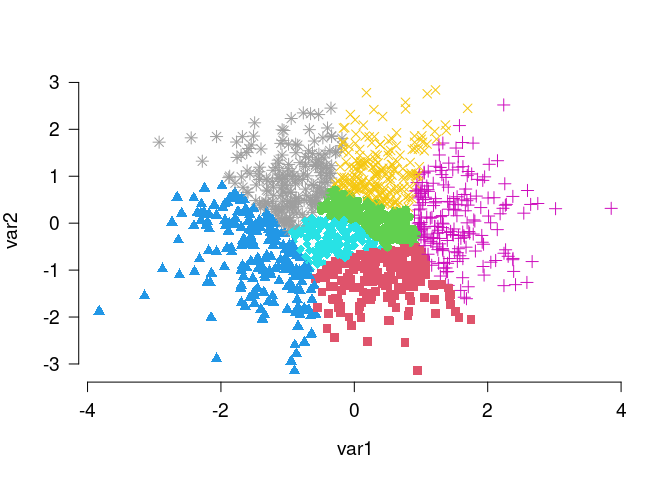
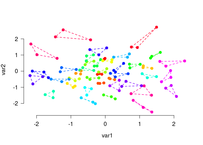
The function matching() is very similar, but is usually used to find small groups of similar elements, e.g., triplets as in this example:
# Generate random data and find triplets of similar elements:
N <- 120
lds <- data.frame(var1 = rnorm(N), var2 = rnorm(N))
triplets <- matching(lds, p = 3)
plot_clusters(
  lds,
  clusters = triplets,
  within_connection = TRUE,
  show_axes = TRUE
)
Questions and suggestions
If you have any question on the anticlust package or find some bugs, I encourage you to open an issue on the Github repository.