Bicriterion iterated local search heuristic
Source:R/bicriterion_iterated_local_search_call.R
bicriterion_anticlustering.RdThis function implements the bicriterion algorithm BILS for anticlustering by Brusco et al. (2020; <doi:10.1111/bmsp.12186>). The description of their algorithm is given in Section 3 of their paper (in particular, see the Pseudocode in their Figure 2). It also implements some extensions to the bicriterion approach for anticlustering described in Papenberg, Breuer, et al. (2025).
Arguments
- x
The data input. Can be one of two structures: (1) A feature matrix where rows correspond to elements and columns correspond to variables (a single numeric variable can be passed as a vector). (2) An N x N matrix dissimilarity matrix; can be an object of class
dist(e.g., returned bydistoras.dist) or amatrixwhere the entries of the upper and lower triangular matrix represent pairwise dissimilarities.- K
How many anticlusters should be created. Alternatively: (a) A vector describing the size of each group, or (b) a vector of length
nrow(x)describing how elements are assigned to anticlusters before the optimization starts.- R
The desired number of restarts for the algorithm. By default, both phases (MBPI + ILS) of the algorithm are performed once. See details.
- W
Optional argument, a vector of weights defining the relative importance of dispersion and diversity (0 <= W <= 1). See details.
- Xi
Optional argument, specifies probability of swapping elements during the iterated local search. See examples.
- dispersion_distances
A distance matrix used to compute the dispersion if the dispersion should not be computed on the basis of argument
x.- average_diversity
Boolean. Compute the diversity not as a global sum across all pairwise within-group distances, but as the sum of the average of within-group distances.
- init_partitions
A matrix of initial partitions (rows = partitions; columns = elements) that serve as starting partitions during the iterations of the first phase of the BILS (i.e., the MBPI). If not passed, a new random partition is generated at the start of each iteration (which is the default behaviour).
- return
Either "paretoset" (default), "best-diversity", "best-average-diversity", "best-dispersion". See below.
Value
By default, a matrix of anticlustering partitions
(i.e., the approximated pareto set). Each row corresponds to a
partition, each column corresponds to an input element. If the
argument return is set to either "best-diversity",
"best-average-diversity", or "best-dispersion", it only returns one
partition (as a vector), that maximizes the respective objective.
Details
The bicriterion algorithm by Brusco et al. (2020) aims to
simultaneously optimize two anticlustering criteria: the
diversity_objective and the
dispersion_objective. It returns a list of partitions
that approximate the pareto set of efficient solutions across both
criteria. By considering both the diversity and dispersion, this
algorithm is well-suited for maximizing overall within-group
heterogeneity. To select a partition among the approximated pareto
set, it is reasonable to plot the objectives for each partition
(see Examples).
The arguments R, W and Xi are named for
consistency with Brusco et al. (2020). The argument K is
used for consistency with other functions in anticlust; Brusco et
al. used `G` to denote the number of groups. However, note that
K can not only be used to denote the number of equal-sized
groups, but also to specify group sizes, as in
anticlustering.
This function implements the combined bicriterion algorithm BILS,
which consists of two phases: The multistart bicriterion pairwise
interchange heuristic (MBPI, which is a local maximum search
heuristic similar to method = "local-maximum" in
anticlustering), and the iterated local search (ILS),
which is an improvement procedure that tries to overcome local
optima. The argument R denotes the number of restarts of
the two phases of the algorithm. If R has length 1, half of
the repetitions perform the first phase MBPI), the other half
perform the ILS. If R has length 2, the first entry
indicates the number of restarts of MBPI the second entry indicates
the number of restarts of ILS. The argument W denotes the
relative weight given to the diversity and dispersion criterion in
a given run of the search heuristic. In each run, the a weight is
randomly selected from the vector W. As default values, we
use the weights that Brusco et al. used in their analyses. All
values in W have to be in [0, 1]; larger values indicate
that diversity is more important, whereas smaller values indicate
that dispersion is more important; w = .5 implies the same
weight for both criteria. The argument Xi is the probability
that an element is swapped during the iterated local search
(specifically, Xi has to be a vector of length 2, denoting the
range of a uniform distribution from which the probability of
swapping is selected). For Xi, the default is selected
consistent with the analyses by Brusco et al.
If the data input x is a feature matrix (that is: each row
is a "case" and each column is a "variable"), a matrix of the
Euclidean distances is computed as input to the algorithm. If a
different measure of dissimilarity is preferred, you may pass a
self-generated dissimilarity matrix via the argument x. The
argument dispersion_distances can additionally be used if
the dispersion should be computed on the basis of a different
distance matrix.
As of anticlust version 0.8.6, this function includes some extensions
to the original BILS by Brusco et al. (2020). These extensions are are
implemented through the optional arguments dispersion_distances,
average_diversity, init_partitions, and return, and
were described in Papenberg, Breuer, et al. (2025).
If these arguments are not changed, the function performs the "vanilla" BILS
as described in Brusco et al. If multiple init_partitions are given,
ensure that each partition (i.e., each row ofinit_partitions) has the exact
same output of table.
Note
For technical reasons, the pareto set returned by this function has a limit of 500 partitions. Usually however, the algorithm usually finds much fewer partitions. There is one following exception: We do not recommend to use this method when the input data is one-dimensional where the algorithm may identify too many equivalent partitions causing it to run very slowly (see section 5.6 in Breuer, 2020).
References
Brusco, M. J., Cradit, J. D., & Steinley, D. (2020). Combining diversity and dispersion criteria for anticlustering: A bicriterion approach. British Journal of Mathematical and Statistical Psychology, 73, 275-396. https://doi.org/10.1111/bmsp.12186
Breuer (2020). Using anticlustering to maximize diversity and dispersion: Comparing exact and heuristic approaches. Bachelor thesis.
Papenberg, M., Breuer, M., Diekhoff, M., Tran, N. K., & Klau, G. W. (2025). Extending the Bicriterion Approach for Anticlustering: Exact and Hybrid Approaches. Psychometrika. Advance online publication. https://doi.org/10.1017/psy.2025.10052
Examples
# Generate some random data
M <- 3
N <- 80
K <- 4
data <- matrix(rnorm(N * M), ncol = M)
# Perform bicriterion algorithm, use 200 repetitions
pareto_set <- bicriterion_anticlustering(data, K = K, R = 200)
# Compute objectives for all solutions
diversities_pareto <- apply(pareto_set, 1, diversity_objective, x = data)
dispersions_pareto <- apply(pareto_set, 1, dispersion_objective, x = data)
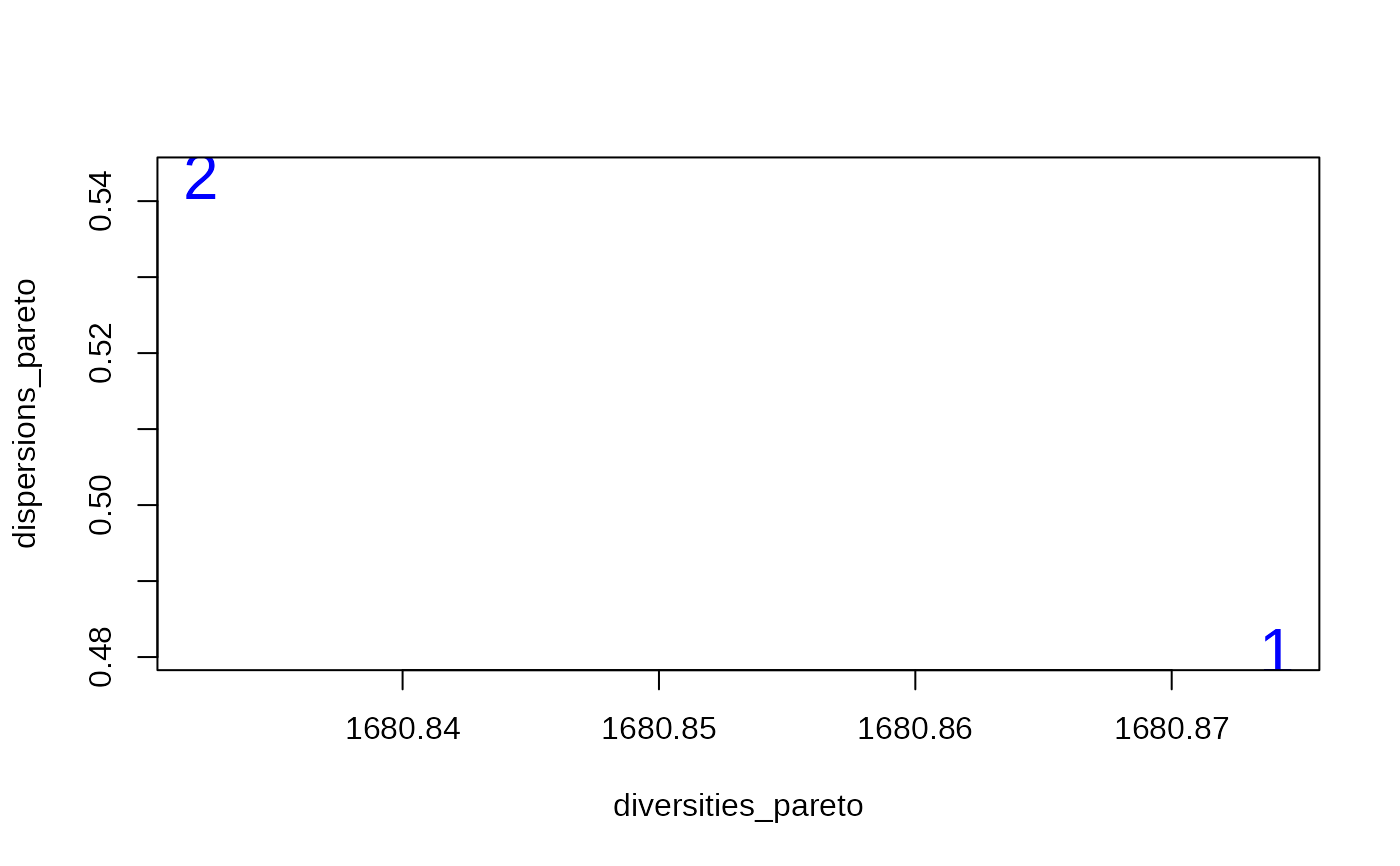
# Plot the pareto set
plot(
diversities_pareto,
dispersions_pareto,
col = "blue",
cex = 2,
pch = as.character(1:NROW(pareto_set))
)
 # Get some random solutions for comparison
rnd_solutions <- t(replicate(n = 200, sample(pareto_set[1, ])))
# Compute objectives for all random solutions
diversities_rnd <- apply(rnd_solutions, 1, diversity_objective, x = data)
dispersions_rnd <- apply(rnd_solutions, 1, dispersion_objective, x = data)
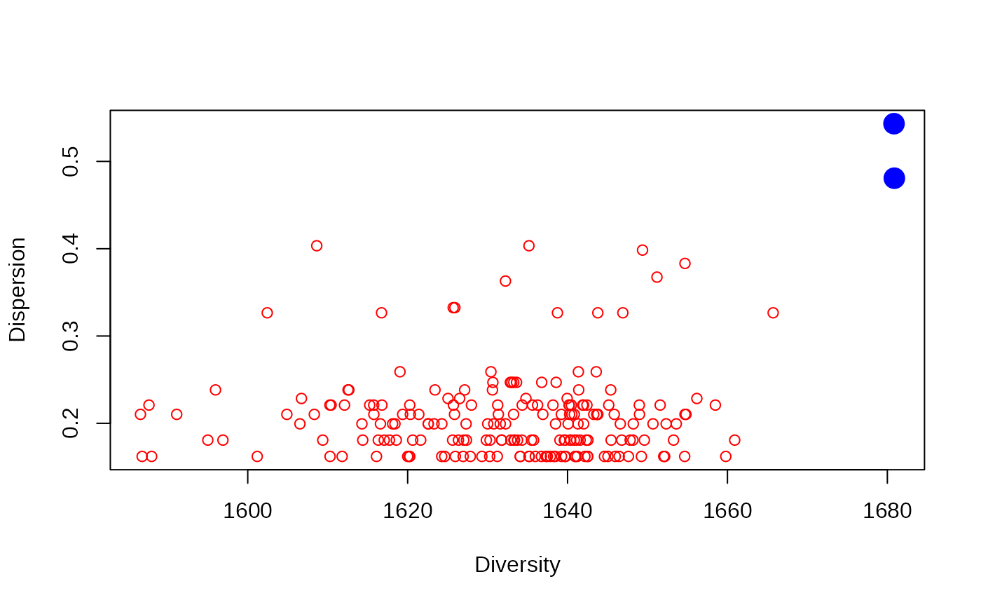
# Plot random solutions and pareto set. Random solutions are far away
# from the good solutions in pareto set
plot(
diversities_rnd, dispersions_rnd,
col = "red",
xlab = "Diversity",
ylab = "Dispersion",
ylim = c(
min(dispersions_rnd, dispersions_pareto),
max(dispersions_rnd, dispersions_pareto)
),
xlim = c(
min(diversities_rnd, diversities_pareto),
max(diversities_rnd, diversities_pareto)
)
)
# Add approximated pareto set from bicriterion algorithm:
points(diversities_pareto, dispersions_pareto, col = "blue", cex = 2, pch = 19)
# Get some random solutions for comparison
rnd_solutions <- t(replicate(n = 200, sample(pareto_set[1, ])))
# Compute objectives for all random solutions
diversities_rnd <- apply(rnd_solutions, 1, diversity_objective, x = data)
dispersions_rnd <- apply(rnd_solutions, 1, dispersion_objective, x = data)
# Plot random solutions and pareto set. Random solutions are far away
# from the good solutions in pareto set
plot(
diversities_rnd, dispersions_rnd,
col = "red",
xlab = "Diversity",
ylab = "Dispersion",
ylim = c(
min(dispersions_rnd, dispersions_pareto),
max(dispersions_rnd, dispersions_pareto)
),
xlim = c(
min(diversities_rnd, diversities_pareto),
max(diversities_rnd, diversities_pareto)
)
)
# Add approximated pareto set from bicriterion algorithm:
points(diversities_pareto, dispersions_pareto, col = "blue", cex = 2, pch = 19)